
Stop counting indexes
Fifty extra indexes don't slow down your writes, but one vector field slows them down 11x. I wanted to figure out why valkey-search behaves this way, and it wasn't what I expected.
 Allen Helton
Free text search is a beast. Sometimes a user will type in a description of what they’re looking for, like “wireless earbuds under $100,” and other times they’ll copy/paste a SKU for an item they’re replacing. Both are completely valid use cases, but the former requires a vector search and the latter relies on lexical matching. I’ve been spending a lot of time in valkey-search trying to handle both. As you can probably imagine, one index doesn’t cut it, but two indexes on the same keys can.
But doubling the number of indexes I was using made me nervous. I didn’t know what impact that would have on performance. I’m using Valkey because I needed ultra-low latency, I didn’t want to shoot myself in the foot trying to be clever.
And yes, going from one to two indexes is probably not a big deal. But indexes have a way of piling up. You create one to filter products by category, then add price to it a month later, then the search team wants a vector field, then the payment team indexes their keys, then fulfillment indexes theirs. Before you know it, there are a dozen FT.CREATE statements in the repo with no single owner.
My instinct tells me that performance scales inversely with the count. Every index in valkey-search subscribes to a key prefix. When you write a matching key, that index gets an entry in a mutation queue, and your client stays blocked until every entry is processed. That’s what gives you read-after-write consistency. If you have a dozen indexes, you also have a dozen entries, and a dozen times the wait. Right?
So I built a benchmark to see how much additional indexes cost in valkey-search. And I discovered I was very wrong.
The setup
The server was an r7i.4xlarge with 8 physical cores, running Valkey 9.1.1 and valkey-search 1.2.1. valkey-search sized its own writer pool to 8 threads. I turned persistence off, because I didn’t need a background save forking mid-run throwing a wrench into my latency numbers. Load came from a separate c7i.8xlarge in the same placement group, over 384 connections.
Every write is the same 4.6KB product hash that includes a category, a price, a SKU, a title, a description, and a 1024-dimension embedding. The load generator sends on a schedule and times each request from when it was supposed to go out, not when it managed to (more on this later). Every point runs for 25 seconds, three times, and I capture the median.
Do idle indexes cost anything?
As I mentioned earlier, indexes subscribe to a key prefix. If a key is upserted that doesn’t match on an index, does that slow things down? In other words, my test here determines if the existence of indexes slows down the performance of others.
I ran the same write workload against product: keys in two setups: one index on product:, and another one with the same index plus fifty more indexes on unrelated prefixes.
| setup | sustained writes/sec | p99 @ 2,000/s |
|---|---|---|
1 index on product: | 32,000 | 2.18ms |
| same index + 50 on other prefixes | 32,000 | 2.17ms |
Nice! I couldn’t measure a difference between them at any rate I tried.
This is because the prefix subscriptions live in a trie. When you write product:88213, valkey-search walks the trie and only notifies the indexes whose prefix matches. An index subscribed to orders: doesn’t hear about it. FT.INFO idx:other0 reports a field called mutation_queue_size, and across the entire run it never left zero, which validates the promise of the trie architecture.
So that hodgepodge of indexes in your repo isn’t what’s slowing your writes down. Only indexes whose prefix matches the keys you write are in the path at all.
The impact of matching indexes
So what’s the performance impact of having multiple matching indexes? I ran the same workload again, this time adding multiple identical indexes directly on the product: prefix.
indexes on product: | writes/sec | indexing jobs/sec |
|---|---|---|
| 0 | 80,000 | 0 |
| 1 | 33,636 | 33,636 |
| 2 | 20,000 | 40,000 |
| 4 | 16,818 | 67,272 |
Every matching index gets an indexing job, and the write isn’t done until all of them are. To figure this out, I took Valkey’s search_ingest_hash_keys counter and divided by the writes that completed in the same window. I took this number and multiplied it by the write rate to calculate the indexing jobs/sec column.
The expensive part, naturally, is switching indexing on in the first place. Going from zero indexes to one cost me 58% of my write rate. The second index cost another 41%. Doubling from two to four only cost 16%. Each additional index cost less than the previous one.
Adding indexes pulls more total indexing work per second out of the same server, 33,636 jobs a second at one index and 67,272 at four. So one or two indexes clearly weren’t saturating the writer pool, because it eventually went on to do twice the work.
Indexing jobs fan out across a pool sized to your physical core count, and the blocked-client handles collapse into a single block on your connection. The write waits for the slowest single job, which is why four indexes don’t cost four times what one does.
Unfortunately I don’t know what the limiting factor is. My hunch is that it’s the per-index bookkeeping that happens on the main thread before a job reaches the pool, but I didn’t measure that, so 🤷.
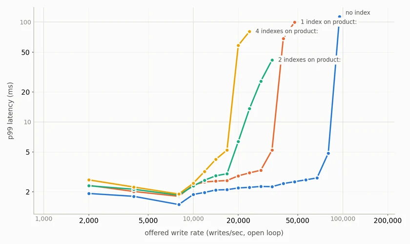
NOTE - Adding matching indexes won’t appear to add latency until it’s too late. At 2,000 writes/sec, one index and four indexes were within a millisecond of each other. You won’t catch it watching p99 on a healthy system, because what you’re spending is headroom. You find out it’s gone when you need it.
Vector fields hit different
The benchmarks above use TAG and NUMERIC fields, just the normal filter field types. So I went back to the first benchmark, added a single 1024-dimension HNSW vector field to the one-index setup, and re-ran it to find some staggering results.
32,000 writes per second became 2,828. 🤯
That’s an 11x difference in throughput because of a single field. My napkin math says that’s 2-3 milliseconds of CPU per vector insert spread across eight writer threads. To make matters worse, the performance cliffs. I increased the rate on my benchmark by ~40%, and the wheels fell off.
| offered writes/sec | p99 | writer queue depth |
|---|---|---|
| 2,828 | 5.65ms | 4 |
| 4,000 | 2,046ms | 376 |
The performance hit goes from five milliseconds to two seconds. The queue went from basically empty to 376 entries deep, and it stayed there for every rate I tried above that. You’re either under the line and fine, or over it and everything is late. If you’re capacity planning, be sure to check whether an index on your hot prefix has a vector field.
Do vector fields affect other matching indexes?
Back to the search feature I was building that required two indexes. A single index can’t do both jobs because of stop words. The text pipeline is configured for the entire index, and it splits words on punctuation before dropping anything in the stop word list. So IT-500 becomes it and 500, it is a stop word, so just 500 is added to the index. Turning on NOSTOPWORDS means your description field will index every the, is, and, and it (plus a lot more) in the catalog. So we need two indexes to have it turned on for one and off for the other.
But that made me wonder what the second index costs when the first one has a vector field. We saw how much of a hit it made to throughput in our earlier benchmarks.
| configuration | sustained writes/sec | p99 |
|---|---|---|
| semantic (TAG + NUMERIC + HNSW) | 2,828 | 5.29ms |
| semantic + exact (TEXT, NOSTOPWORDS) | 2,828 | 5.44ms |
About a three percent difference. The exact match index processed 141,408 text fields during the benchmark run. Both mutations hit the pool together, the write waits for the slower one (the vector). So if you’re already paying the HNSW tax, the lexical index has essentially no additional latency.
My takeaways
So it turns out I was asking the wrong question when I started this experiment. I thought the number of indexes I had was going to slow performance down to a crawl. But it doesn’t. The real question is what fields are inside the indexes that match your keys? Which is a relief, when I think about it.
I also learned a couple of things about benchmarking while I was busy answering the wrong question. 😅
Every sustained writes/sec number in this post could have been bigger. At the top rung of my ladder, the no-index setup completed 128,000 writes a second (but my tables show 80,000). At that run rate, it was making every request wait 1.9 seconds in a queue first. A server running at full utilization drains as fast as it fills, so throughput looks perfect, but at a cost to latency. So the number I used in every table is the highest rate where p99 stayed within reason.
It took me three runs to believe what I saw in that four-row table early in this post. The first run stepped the rate by 1.4x per rung, which put two indexes and four indexes on the same 16,000 rung. Which at first made me think indexes three and four had no performance implications. But in reality, they had both fallen apart somewhere between rungs and the ladder couldn’t show me where. So I re-ran it with 1.19x steps and got a cleaner separation. Then I noticed that ladder started at 14,000, which is already well up the curve, so it never measured what latency looks like when the server is idle. My rule for picking a sustainable rate is relative to that idle number, which meant the second run was grading itself on a curve. The third run started at 2,000 and is the one in the table. A rate ladder can’t resolve a difference smaller than its own step, and it can’t tell you where the knee is if it never saw the flat part before it.
Try it yourself
I have the benchmark, scripts, and results available in GitHub. If you want to check my numbers (or disagree with them!), please do and let me know what you find.
If you want to run the same tests on your own Valkey cluster, you can run these three commands:
FT.INFO <index> # shows mutation_queue_size (write backlog) for the specified index
INFO search # shows search_writer_queue_size for the whole pool
CONFIG SET search.info-developer-visible yes # unlocks per-field-type counters like search_ingest_field_vector
It’s cheap to experiment with your existing clusters because these mutations are reversible. FT.DROPINDEX is instant and your data was never in the index to begin with. Add a shape, measure it, then discard it.
Happy coding!