Pop quiz: how many requests per second can your cache take before it stops meeting your latency SLO?
Chances are good you don’t know the answer, and that’s not a knock on you. It’s a genuinely hard number to come by. The standard tool for this is valkey-benchmark, and it’s great at exactly one thing: you point it at a server, you hammer it with some commands at full speed, and it prints a throughput number at the end. That number tells you the box is alive and roughly how fast it goes flat out.
From a production standpoint, that’s not as useful as it sounds.
How does the p999 hold up under an 80:20 read/write mix when half the requests land on hot keys? What does the tail look like at the rate you actually plan to run? How much headroom do you have before the SLO breaks? Was that latency spike at 10:32 a fluke or the ceiling? A single summary number printed after a sixty-second run can’t answer any of those, because it threw away the useful bits on the way to computing the average.
valkey-lab was built to answer these questions.
It’s a high-performance Valkey and Redis benchmark that uses io_uring for kernel-bypassed I/O, per-connection pipelining, and multi-threaded workers. The defaults are deliberately familiar. Run it without any arguments:
📄
valkey-lab
and you get a sixty-second run against localhost:6379 with an 80:20 GET/SET ratio and a million keys. Same shape as the tool you already know, same short flags (-h, -p, -c, -P, -r). The interesting part starts once you begin asking harder questions.
Saturation search: the headroom number, found for you
Here’s how you find your headroom number today, by hand. You run a benchmark at some rate, read the p999, decide it looks healthy, bump the rate, run it again, read it again. You do this five or ten times, squinting at each result, trying to find the rate where the tail skyrockets. Somewhere in that loop you lose track of which run had which config. Eventually you settle on a number you’re “pretty sure” is right and plan capacity around it. valkey-lab does that whole search for you with one command.
📄
valkey-lab saturate --slo-p999 1ms -c 16 -P 32
A synthetic benchmark might say a cache can handle 2M requests per second. But when you add a realistic read/write mix, hot keys, and a warm cache, your p999 suddenly crosses your SLO at 1.2M. Technically speaking, the server is still processing 2M requests per second, but the usable ceiling is significantly lower.
saturate starts issuing requests at whatever is provided in --start-rate (or 1000 if not provided) and multiplies the request rate by the --step factor on every step. The default step is 1.05, so the load compounds over time. Each step holds its rate for a sample window, measures the full percentile spread, and checks it against your SLO. The moment a percentile crosses the line, the ramp stops and reports the last rate that held.
When a step fails, valkey-lab tells you how it failed, either throughput-limited or latency-exceeded, which helps you tune your clusters more accurately.
Throughput-limited means the server couldn’t generate the requested rate at all. It topped out below the target. That’s a capacity problem: you need more CPU, more shards, or a different topology.
Latency-exceeded means the server kept up with the rate, but the tail blew past the SLO. The server can sustain the requested rate, but something in the path is introducing tail spikes under load. Could be a hot key, a GC pause, a scheduler stall, network jitter. You fix that by chasing the spike, and adding hardware won’t help.
So based on your failure, your mitigation strategy varies wildly. And it would be impossible to know which one to pursue if all you had was the throughput number.
Averages hide the interesting failures
The next problem surfaces when the benchmark completes. Summary statistics hide the behavior you’re usually trying to find. If your p999 was 312µs for fifty-nine seconds and 4.2 ms for one second, the run-level p999 still looks fine. The spike is the important part that you need to focus on.
valkey-lab streams one row per second with the full latency spread:
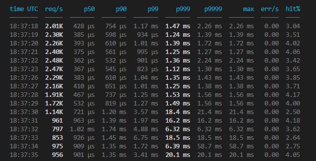
Every major percentile from p50 to p99.99 plus the max, the error count, and the cache hit rate, all per second. A spike that lasts one second appears as one row with a tall tail, a vast improvement over the executive summary at the end of a run. When you need it machine-readable instead, –output json gives you newline-delimited JSON you can pipe straight into something else, and –output quiet collapses the whole run to a single summary line.
Make the benchmark look like your workload
There’s an important gotcha with the saturation number, or any benchmark number. A ceiling is only as good as the load that produced it, and the default load most tools run is unrealistic.
Think about what a stock benchmark actually does. It sends all reads, or close to it, because a 100% GET run posts the biggest number (or it’s the easiest to simulate). It picks keys uniformly at random, so every key is equally cold and nothing is ever hot. It runs flat out, measuring throughput at saturation. And it normally starts against an empty cache. Now think about your production traffic. It’s a read-write mix. It has hot keys, with a small fraction of the keyspace taking most of the requests. And the cache is warm. Every one of those differences takes away from the realism of the benchmark run.
valkey-lab addresses each one of these gaps. Set the real read-write split with -r so you’re measuring the write path your cache actually carries. Turn on –distribution zipf so a small fraction of keys receives most of the traffic, like production systems often do. Uniform access patterns avoid contention and hide the behavior of your actual hot paths.
Pin the load with –rate-limit to track latency at the rate you plan to run. And warm the cache with –prefill, or model a read-through cache that fills on miss with –backfill, so a GET benchmark measures hits the way production would.
📄
valkey-lab --prefill -r 100:0 --distribution zipf -c 16 -P 32
Stack those and the ceiling you measure is a ceiling that meaningfully tracks production. There’s more depth when you need it, warmup tuning, RESP3, pinning workers to cores with –cpu-list, TLS, full TOML configs, but the move that matters is making the four big assumptions match your reality before you trust the number.
Getting the important data from a run
Now that we have realistic benchmark data, we have to make sure it’s useful after the run ends.
--parquet results.parquet saves the full dataset to disk. It stores the full metric set per snapshot: the counters, the gauges, and the latency distributions as actual nanosecond histograms. Combine this with the visualization functionality in valkey-lab, and you have a rich experience that lets you dig into every tiny detail.
📄
valkey-lab --parquet results.parquet
valkey-lab view results.parquet
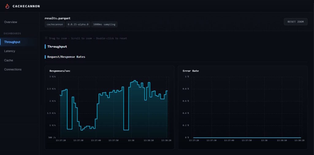
view opens an interactive dashboard against the file, with a synchronized time axis you can zoom and pan through dimensions like throughput, hit rate, error rate, and latency split out by GET, SET, and combined, all on a log scale. Scrub to the exact second p999 jumped and read every other metric in that same window.
One use case for this is regression testing. Because every run is a Parquet file with the same schema, runs are directly comparable to each other. Benchmark before a Valkey upgrade and after, and the question “did this move my tail latency” is easily answered with a diff. The viewer is one way to read these files, but using your own queries is another easy way to act on changes in performance. DuckDB, pandas, and Polars all read Parquet directly, so a few lines of SQL across a directory of runs is a regression suite for cache performance. Point DuckDB at a folder of recorded runs and let it compute peak throughput per file:
📄
SELECT
  filename,
  max(responses_received) AS total_responses,
  max(request_errors)     AS errors
FROM read_parquet('runs/*.parquet', filename = true)
GROUP BY filename
ORDER BY filename;
That is a before-and-after table for every benchmark you have ever saved, built from data you already recorded.
Another use case for the Parquet output is root cause analysis. A spike on the latency chart tells you when something went wrong, not why. Point view at a Rezolus capture from the server or the client and it overlays system telemetry, CPU utilization, network, scheduler behavior, aligned to the same benchmark timeline. When a p999 spike lines up exactly with a scheduler stall or a network hiccup on the axis above it, you have your answer as simple as that.
Stop guessing
Back to the pop quiz. The reason it’s so hard to answer is that traditionally the tool you use to measure max RPS reports a summary and throws the important bits away. valkey-lab changes the approach. It remembers the mix, the hot keys, the per-second tail, and records your runs so you can come back to them. The headroom number that used to take an afternoon of manual ramping is now a single command, and it comes with the failure mode attached so you know what to do about it.
valkey-lab is built on top of cachecannon, inheriting its workload generation, saturation search, telemetry collection, and analysis capabilities. It needs Linux for io_uring (kernel 6.0+) and builds with Rust, under your choice of Apache-2.0 or MIT. Here is the whole getting-started path:
📄
cargo install --path . --bin valkey-lab
valkey-lab saturate --slo-p999 1ms
Run that against a Valkey server and see what number comes back. Stop asking “how fast can my cache go” and start asking “how fast can it go before my production workload breaks?” That’s the number you capacity-plan around if you want predictable systems at 3 AM.